While the agronomic and economic benefits of regulated deficit irrigation (RDI) strategies have long been established in red wine grape varieties, spatial variability in water requirements across a vineyard limits their practical application. This study aims to evaluate the performance of an integrated methodology—based on a vine water consumption model and remote sensing data—to optimize the precision irrigation (PI) of a 100-ha commercial vineyard during two consecutive growing seasons. In addition, a cost-benefit analysis (CBA) was conducted of the tested strategy. Using an NDVI generated map, a vineyard with 52 irrigation sectors and the varieties Tempranillo, Cabernet and Syrah was classified in three categories (Low, Medium and High). The proposed methodology allowed viticulturists to adopt a precise RDI strategy, and, despite differences in water requirement between irrigation sectors, pre-defined stem water potential thresholds were not exceeded. In both years, the difference between maximum and minimum water applied in the different irrigation sectors varied by as much as 25.6%. Annual transpiration simulations showed ranges of 240.1–340.8 mm for 2016 and 298.6–366.9 mm for 2017. According to the CBA, total savings of 7090.00 € (2016) and 9960.00 € (2017) were obtained in the 100-ha vineyard with the PI strategy compared to not PI. After factoring in PI technology and labor costs of 5090 €, the net benefit was 20.0 € ha −1 in 2016 and 48.7 € ha −1 in 2017. The water consumption model adopted here to optimize PI is shown to enhance vineyard profitability, water use efficiency and yield.
Avoid common mistakes on your manuscript.
In viticulture, maximum incomes are not always achieved with maximum yield but by maintaining a certain balance between yield and berry composition. It is evident that judicious irrigation contributes to improving water use efficiency (WUE), controlling canopy vigor and enhancing grapevine berry composition (Chaves et al. 2007). In particular, the adoption of regulated deficit irrigation (RDI) strategies has been widely used in red grape varieties as a water saving strategy as well as to enhance berry composition attributes (Roby et al. 2004; Santesteban et al. 2011; Basile et al. 2011; Casassa et al. 2015). For instance, Basile et al. (2011) reported that in cv. ‘Cabernet Sauvignon’, berry composition improved when mild stress was applied between fruit set and veraison, and with moderate to severe water stress in post-veraison. The precise adoption of RDI requires careful selection of the moment, intensity and duration of the water deficit application (Conesa et al. 2018). This can only be properly achieved with a precise knowledge of the seasonal sensitivity of grapevine to water stress and using physiological plant-based tools such as the leaf/stem water potential as indicators of water stress (Girona et al. 2006, 2009). However, the main drawback when adopting these irrigation strategies in commercial vineyards is that it is extremely complicated to attain the same desired water stress level in all the subzones within a vineyard. The spatial differences in soil properties and topography reflect changes in water requirements across a vineyard, thereby limiting the efficient use of water. If irrigation is uniformly applied without considering spatial differences in water requirements there is a risk of a very significant productive and quality reduction in subzones where water stress is excessive. Equally, in overwatered subzones, the intended berry composition quality levels may not be achieved. To succeed with the practical application of RDI strategies at field level, it is first necessary to consider the following three aspects: (i) to characterize within-field soil spatial variability, since not all soils retain or provide water to the plant at the same rates. Currently, an appropriate procedure to map the spatial variation of soil properties is through the measurement of apparent soil electrical conductivity (ECa), using electromagnetic induction conductivity instrumentation such as the commercial Veris 3100 sensor system (Veris Technologies, Salina, KS) or EM-38 sensors (Geonics Ltd., Mississauga, Ont, Canada) (Corwin and Lesch 2003; Abdy et al. 2008). Good correlations between ECa and soil salinity, soil water content and soil texture have been widely reported (Moral et al. 2010; Uribeetxebarria et al. 2018); (ii) to adapt secondary irrigation networks according to the natural variability of soils. Several studies have proposed different methodologies to re-design the irrigation sectors based on yield map time-series, soil properties or spectral vegetation indices (Bellvert et al. 2012; Martínez-Casasnovas et al. 2009); and (iii) to obtain appropriate physiological knowledge about the optimal water stress thresholds of each variety and the optimal phenological moment to achieve the best balance between yield and berry composition.
Until now, the most commonly used irrigation practice by viticulturists has been based on a simple water balance approach, where crop evapotranspiration (ETc) is calculated with standard crop coefficients (Kc) and the soil water content with data from soil moisture sensors, which are installed in a particular representative place of the vineyard. Then, irrigation scheduling is uniformly applied in the whole vineyard. Some large modernized wineries also complement this methodology with information gathered from other plant-based sensors (Jones 2004; Eastham and Gray 1998; Ginestar et al. 1998a, b). However, the use of any plant-based or similar indicator for scheduling irrigation requires the definition of reference or threshold values, beyond which irrigation is necessary. In addition, a general limitation to plant-based methods is that they do not usually give information on ‘how much’ irrigation to apply at any one time, only on whether irrigation is needed or not (Jones 2004). Thus, irrigation prescriptions which use such tools when RDI is to be imposed have to be determined through trial and error methods.
The development of new precision irrigation (PI) scheduling systems aims to quantify the irrigation needs at spatial level according to the actual vine water status and with the goal of achieving a specific target. For this to be accomplished, the new challenge for PI in viticulture is to use a series of technological procedures in an integrated manner to individually resolve the three requirements described above for the implementation for RDI strategies, but which, without a clear link between them, cannot be commercially applied. Such new methodology needs to be properly integrated and can, for instance, be based on the use of geographic information systems (GIS), remote sensing, crop simulation models and irrigation management knowledge. These integrated procedures must also consider the criteria of the seasonal sensitivity of vines to water stress, and to have a reasonable cost/benefit ratio. A priori, the proper adoption of RDI strategies in red grape varieties seems profitable. According to the Raïmat winery (Spain), the difference in the rate of return between standard and high-quality berries can be as much as 310 € tn −1 . This means that in a vineyard with an average yield of 8–10 tn ha −1 , an income of 2700 € ha −1 can be obtained. In addition, improvements in water use efficiency (WUE) can also reduce water and electricity costs by up to 20%. If the actual average cost of energy and water is 320 € ha −1 , a potential saving of 20% corresponds to 64 € ha −1 .
In view of the above, the first objective of the present study was to develop a decision-oriented vine water consumption model for scheduling irrigation. This model has to be able to simulate the actual amount of water evapotranspirated per vine and to determine the necessary amount of water to be applied when different irrigation strategies (either full-irrigation or RDI) are to be imposed. The second objective was to demonstrate the performance of an integrated methodology for optimizing the precise irrigation of a 100-ha commercial vineyard based on use of the developed vine water consumption model and remote sensing data. Finally, a cost-benefit analysis (CBA) was performed to evaluate the profitability of conducting a PI management using the abovementioned integrated methodology.
It was hypothesized that the implementation of RDI in a 100-ha vineyard with notable differences in vine water requirements can only be successfully adopted with a series of integrated technological procedures based on the use of remote sensing as a tool to identify spatial variability and to classify irrigation sectors with similar characteristics, and a vine water consumption model capable to quantify irrigation needs according to actual and targeted vine water status. The proper adoption of this procedure could enhance vineyard profitability, water use efficiency and yield.
The model developed in this study uses CropSyst principles (http://modeling.bsyse.wsu.edu/CS_Suite_4/CropSyst/index.html) (Stöckle et al. 2003) and has been recently adapted for different deciduous trees (Marsal et al. 2013, 2014). For this study, the water consumption model was adapted for grapevines and written in Matlab® language (MATLAB 2014b, The MathWorks, Inc., Natick, Massachusetts, United States) using experimental empirical regression data obtained in previous studies. A diagram of the model with the interrelationships between the different parameters is shown in Fig. 1. Input parameters, such as weather, fraction of intercepted radiation (fIR) and stem water potential (Ψstem), are introduced in the model in separate files. Since this model is run on a daily basis, daily weather data is required (maximum and minimum air temperature, maximum and minimum relative humidity, solar global radiation, rainfall and wind speed). Reference evapotranspiration (ETo) (mm day −1 ) estimation was calculated using the FAO Penman–Monteith equation (Allen et al. 1998).
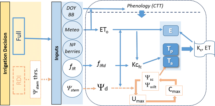
The model allows the user to choose the irrigation strategy to be adopted throughout the growing season: (i) full irrigation (FI) or (ii) RDI. Irrigation prescriptions for FI are calculated based on ET estimates at full transpiring canopy. The stem water potential thresholds (Ψthr) can be defined at different phenological stages when an RDI strategy is adopted. The vegetative growth of the vine is determined as a function of the fraction of the canopy-intercepted solar radiation (fIR), which can be either measured or simulated. Hourly fIR is converted to daily fIR (fIRd) according to the model of Oyarzun et al. (2007). Canopy dimensions (i.e. height, width and length) and geographical coordinates of the vineyard are needed. If fIR measurements are not available, the model can generate simulations of fIRd using a polynomial function based on the accumulation of growing degree-days (GDD).
The phenological stages were defined based on GDD. The accumulation of GDD for each stage was determined with a modified version of the single triangle algorithm method (Zalom et al. 1983; Nendel 2010) described in Prats-Llinàs et al. (2020). The base and upper threshold temperatures were 4 °C and 26 °C, respectively. A maximum heat temperature threshold of 43 °C was also defined. On the occasions when the daily maximum temperature exceeded this threshold, the daily maximum temperature was corrected by applying the relationship between radiation use efficiency (RUE) and temperature described in Prats-Llinàs et al. (2020).
At any stage of canopy development, ET is separated into transpiration (T) and soil evaporation (E) components.
Potential transpiration (Tp) (assuming total canopy cover at full transpiration) is calculated as:
where Kcfc represents the Kc for total canopy cover. In this modelling study, Kcfc includes only vine transpiration and seasonal values were obtained from Picón-Toro et al. (2012) for a mature cv. Tempranillo vineyard as a function of fIRd and thermal time from bud-break.
Soil evaporation (E) is calculated as:
where Ke represents the soil evaporation coefficient and was calculated using experimental data from microlysimeters and as a function of the amount of irrigation water applied in the previous irrigation event and fIRd.
If an RDI strategy is adopted, then it is necessary to enter midday stem water potential (Ψstem) measurements into the model. Using this data, the model calculates the amount of water needed in order to reach the pre-defined Ψthr. Daily values of Ψstem (Ψd) were obtained as an integration of the diurnal course of Ψstem (every 2 h) measurements in TMP Low vines. An empirical polynomial relationship which related Ψstem with Ψd was developed (R 2 = 0.86; n = 40).
$$\psi _>> = > - 0.>\psi _>>> ^>> + >0.>\psi _>>> - >0.>$$Maximum plant hydraulic conductance (Cmax) can be calculated according to an analogue Ohm’s law for full canopy cover as:where Umax is a parameter of the model that represents the maximum water uptake of the crop, Ψsc is the lowest plant water potential that does not limit transpiration, and Ψfc is soil water potential at field capacity. Values for Ψsc change throughout the season, and those adopted in this study coincided with those Ψstem values that had a crop water stress index (CWSI) equal to zero (from − 0.4 to − 1.1 MPa) in the empirical regressions obtained by Bellvert et al. (2015) in different grapevine cultivars. Values of Ψfc were established at − 0.033 MPa. The percentage of reduction due to water stress was calculated as:
$$Reduction \left(\%\right)=1-\frac<<<\Psi >>_-<<\Psi >>_><<<\Psi >>_-<<\Psi >>_>$$where Ψwilt is the lowest plant water potential at wilting point, when transpiration is null. In this study, values of Ψwilt coincide with a CWSI of one (from − 1.1 to − 1.7 MPa) (Bellvert et al. 2015).
Then, actual transpiration (Ta) and evapotranspiration (ETa) can be estimated as:
Based on this, irrigation scheduling was performed on a weekly basis as:
$$> = >\left( >>> \right)/0.>$$where rainfall corresponded to that accumulated during the previous week, and 0.95 is the efficiency of a drip irrigation system.The study was carried out during the growing seasons 2016 and 2017 in a 100-ha organic commercial vineyard located in Raïmat (41°39′50ʺN–0°30′27ʺE) (Lleida, Spain) (Fig. 2a). The vineyard consisted of 52 irrigation sectors ranging between 0.6 and 2.6 ha and planted with the varieties Cabernet Sauvignon (CAB) (38), Tempranillo (TMP) (12) and Syrah (SYR) (2). The area has a typical Mediterranean climate, with dry and hot summers and mild winters. Total rainfall for the growing period 30th March to 16th October was 163.7 mm and 149.8 mm for 2016 and 2017, respectively. The annual accumulated reference evapotranspiration (ETo) was 1100 mm in 2016 and 1400 mm in 2017. The vineyard was planted in 2010 with a 1.6 × 2.5 m spacing distance. The soil texture was silty-loam and the effective soil depth was ~ 0.8 m. The canopy system was trained using vertical shoot positioning (VSP), with a bilateral, spur-pruned cordon located 1.0 m above the ground. Disease control and nutrition vine management were conducted following the wine grape production organic protocol of the ‘Costers del Segre’ Denomination of Origin (Catalonia, Spain) and the Catalan Council of Organic Agricultural Production (Catalan initials: CCPAE).
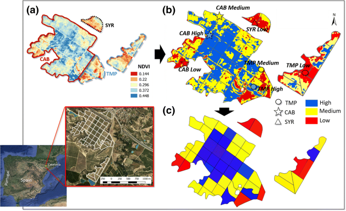
The spatial variability of the vineyard in terms of canopy vigor was determined in July of the 2015 growing season by using airborne high-resolution imagery. Zenith angle images were acquired with an aircraft equipped with a digital multispectral camera (DMSC), which integrates four independent narrow bandwidth spectral filters of 20 nm width (full-width, half-maximum) at the specific band center of 450 (blue), 550 (green), 680 (red), and 780 (near-infrared, NIR) nm. Image resolution is 2048 × 2048 pixel with 14-bit digitalization, with a 24–28 mm fixed focal length yielding an angular field of view (FOV) of 17°. Airborne images were acquired by SpecTerra Services Proprietary Limited (Perth, WA, Australia) under clear sky conditions at ~ 1500 m above ground level yielding images at 0.5 m spatial resolution. Post-flight image processing included a bidirectional reflectance distribution function (BRDF) correction for variations in the sun-sensor-target viewing geometry across each image. The SpecTerra proprietary BRDF correction algorithm preserved the spectral integrity within an image, but produced DN rather than absolute radiance. Therefore, the normalized difference vegetation index (NDVI) was calculated as:
$$NDVI = \frac<Each irrigation sector was classified according to the predominant NDVI category (Fig. 2c). In addition, seven ‘smart points’, which visually corresponded to the most representative location by variety and NDVI category were also identified. These ‘smart points’ were classified as CAB (High, Medium and Low), TMP (High, Medium and Low) and SYR (Low). SYR was classified with only one category because the two irrigation sectors of this variety did not show spatial differences in NDVI. Each ‘smart point’ was composed of six vines, and vine physiological and structural measurements were conducted every one to two weeks and used as inputs of the crop model. The fIR was measured using a portable ceptometer (Accupar Linear PAR, Decagon Devices, Inc., Pullman, WA, USA) placed in a horizontal position at ground level and perpendicular to vines. In order to cover vine spacing, five equally spaced measurements were taken on the shaded side of each vine. The incident radiation above the canopy was determined in an open space adjacent to each vine. Vine structural parameters such as height, and canopy width perpendicular to the row were also measured. Ψstem was measured at noon with a pressure chamber (model 3005; Soil Moisture Equipment Corp., Santa Barbara, ca., USA) according to the recommendations of McCutchan and Shackel (1992). Leaves were wrapped in plastic bags covered with aluminum foil at least one hour before Ψstem was measured. All measurements were taken in less than one hour with four leaves measured at each ‘smart point’. Irrigation prescriptions were then conducted independently in each irrigation sector according to the model outputs. Irrigation was scheduled on a weekly basis and distributed between three to four times a week. Drip emitters of 2.2 L h −1 were used, separated at 0.5 m. The volume of water applied was measured weekly using digital water meters (CZ2000-3M, Contazara, Zaragoza, Spain) located at each ‘smart point’.
Irrigation scheduling consisted of adopting a RDI strategy for all wine grape varieties. For this purpose, different Ψstem thresholds were pre-defined by considering optimal Ψstem values obtained in previous studies in the same varieties (Girona et al. 2009; Basile et al. 2011). Table 1 shows a summary of the pre-defined Ψstem thresholds. Because, at the end of ripening, Syrah berries are more prone than the other varieties to display weight loss due to an insufficient compensation of transpirational water loss by xylem water uptake (Scharwies 2013), the pre-defined Ψstem values for that variety were slightly higher.
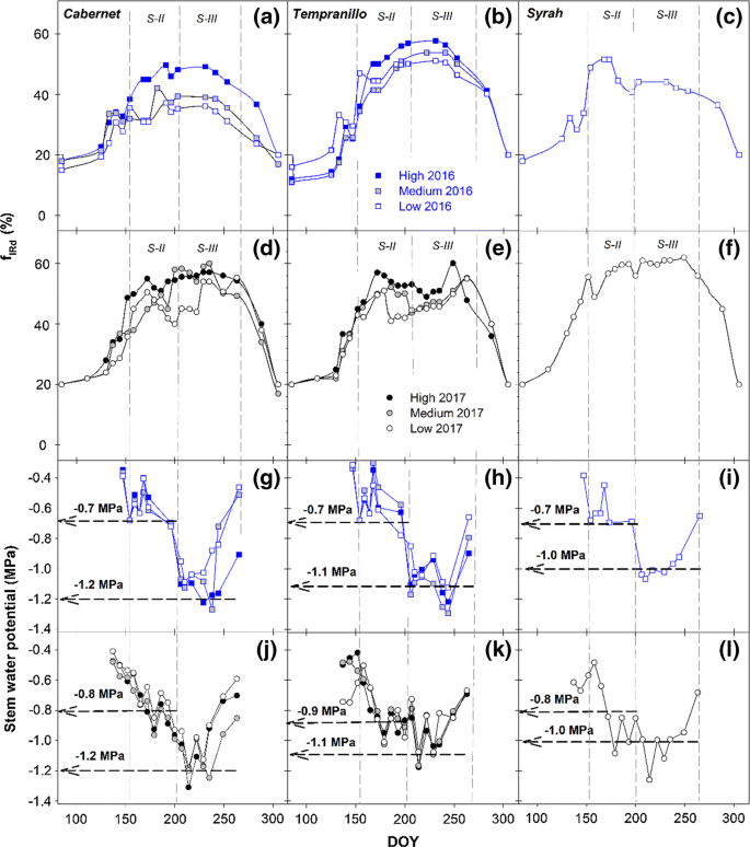
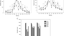
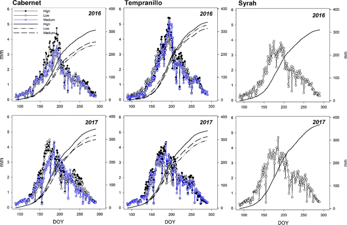
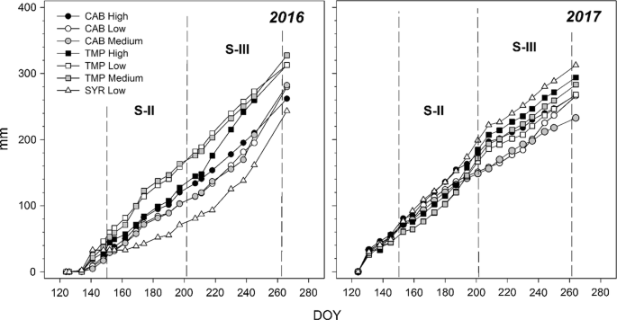
The actual transpiration (Ta) of vines at each ‘smart point’ was simulated during the whole growing season (Fig. 4). In each variety, simulations of Ta indicated significant differences among categories. The seasonal evolution of Ta followed the same pattern as that of vegetative growth, increasing from the beginning of the growing season until reaching maximum values of 4.0–5.5 mm day −1 when fIRd also reached maximum values of 60% (~ DOY 180). Subsequently, Ta started declining, in part due to the adoption of deficit irrigation during post-veraison. Overall, the highest Ta corresponded to vines of the category High, also coinciding with the highest fIRd. Montoro et al. (2016) reported daily Ta rates in cv. ‘Tempranillo’ comparable to those estimated in the present study. Other studies reported peak values of daily Ta of about 2.5 mm day −1 in vines with a canopy light interception of 30% (Intrigliolo et al. 2009). Assuming this canopy light interception was half of that measured in the current study, it confirms that this value was similar to those reported in the present study and which are shown in Fig. 4. In 2016, the highest accumulated Ta was for TMP, ranging from 313.6 mm to 340.8 mm depending on the category (High, Medium or Low). In 2016, SYR had similar values to CAB High, with accumulated Ta of 310.6 mm and 306.2 mm, respectively. In 2017, SYR had the highest accumulated Ta with 366.9 mm, while TMP and CAB had similar values in their respective categories ranging between 296.3 mm and 338.3 mm. Differences between vines in Ta measured at the different ‘smart points’ were calculated with the coefficient of variability (Cv), which ranged from 7.6–12.6%. Table 2 shows that accumulated Ta was about 15–22% lower than potential transpiration (Tp) over the whole growing season. RDI was mostly adopted during post-veraison (growth stage III), with the CWSISIII showing accumulated water stress during that period which ranged from a minimum of 0.17 for SYR Low (2017) to a maximum of 0.36 for CAB High (2016). The results also show that seasonal soil evaporation (E) accounted for 22–24% of total annual ETa. Phogat et al. (2017) reported much higher evaporation values (44–59% of ETa) using a subsurface drip irrigation system. However, the high differences in the amount of rainfall during the growing period between the two study sites may explain these dissimilarities. Other studies (Ferreira et al. 2012; Netzer et al. 2009; Cancela et al. 2012; Montoro et al. 2016) have shown seasonal evaporation varying from 7.4–30% of ETa.
Although Ψstem has been commonly used in research and its advantages extensively demonstrated (Shackel et al. 1997; Girona et al. 2006; Williams 2017), commercial use of this technique is still limited, with only a few wineries currently using this tool in their protocols for scheduling irrigation. The main shortcomings are the initial investment cost and the time that is required to conduct a high number of measurements at midday in order to have a good representation of the vine water status of a whole vineyard. However, the present study demonstrates that, by taking advantage of remote sensing, it is possible to map the spatial variability of a vineyard, to identify zones and irrigation sectors with similar characteristics and to geolocate representative vines within each zone for collection of Ψstem and fIRd measurements. By integrating this information into the developed vine water consumption model, this study has demonstrated that it is possible to conduct effective precision irrigation (PI) management. However, the costs and benefits of applying this methodology only during two consecutive years are still uncertain. Table 3 shows a cost-benefit analysis (CBA) which evaluates the feasibility of using the proposed methodology of the present study in a 100-ha vineyard. To achieve it, the PI management adopted in this study was compared against a not precision irrigation (NPI). The NPI simulated the irrigation prescriptions that a viticulturist should adopt to follow a full-irrigation strategy uniformly applied for the entire vineyard. Therefore, irrigation prescriptions were calculated with the vine water consumption model based on ET estimates at full transpiring canopy (Table 4).
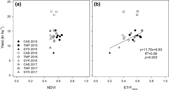
Using both satellite and airborne imagery, significant correlations between spectral vegetation indices and grape yield have been reported in some studies (Sun et al. 2017; Bellvert et al. 2012), but not in others (Bonilla et al. 2015, Anastasiou et al. 2018). In the present study, no statistically significant correlation was obtained in the regression between NDVI and yield (Fig. 7a). For a given range of NDVI values, yield varied in the range 7–22 tn ha −1 . These inconsistencies could be attributable to several causes: (i) it is widely acknowledged that yield is a function of transpiration, and that the latter increases as fIRd increases (Suay et al. 2003). However, this is only true under potential conditions. When water stress occurs, it is because the demand for water exceeds the available amount of water. Thus, it is possible that despite having vines with high canopy vigor (higher water demand), if the amount of water applied is below the water demand, vines can be stressed and therefore have a negative impact on yield; (ii) the spectral vegetation index NDVI has been widely used to identify the spatial and temporal differences in vegetative growth in wine grapes (Balbontín et al. 2017; Sun et al. 2017). However, it is well documented that NDVI tends to saturate at high leaf area index (LAI) values (Barrett and Curtis 1999, Haboudane et al. 2004), resulting therefore in a restriction for quantifying vegetative growth, particularly in relatively dense canopies. In addition, Guillén-Climent et al. (2012) reported the high sensitivity of NDVI to soil background, percentage cover, and sun geometry in heterogeneous orchard canopies. The high sensitivity of NDVI to leaf pigments, spacing distance and training systems also needs to be taken into consideration. Therefore, no unique relationship between NDVI and LAI is universally applicable, and numerous parameters need to be taken into account in order to obtain accurate estimates of LAI. As previously mentioned, yield is a function of crop transpiration. In this respect, Fig. 7b shows a good positive relationship between yield and ETrF_norm for all points except for those of TMP in 2016 which, for a given level of ETrF_norm, tended to have a higher yield. These differences in yield could be attributable to a varying number of clusters as the result of differential cluster thinning.
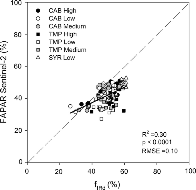
A significant correlation was found between fIRd and FAPAR_S2, with a coefficient of determination (R 2 ) of 0.30 and an RMSE of 0.10 (Fig. 8). Data used in that regression corresponded to the period 15th May to 8th October. Data outside this period was not considered because the presence of inter-row grass cover crop negatively affected the correct estimates of FAPAR_S2. Although the initial results were significant and the estimates of FAPAR_S2 could probably be used as an alternative to in situ fIRd measurement, further research is needed to validate it in heterogeneous crops. FAPAR_S2 is first obtained from radiative transfer models, which depends on canopy structure, vegetation element optical properties and illumination conditions. After, it is used to train a neural network which produces in parallel estimates of the considered biophysical variables. Further research should be focus to train the neural network in vines with different row orientations and training systems. Since most of the cost for conducting a PI management is related to Ψstem and fIR measurements (Table 3), spatio-temporal estimates of FAPAR would considerably reduce the cost and to improve the chances to conduct a PI management.
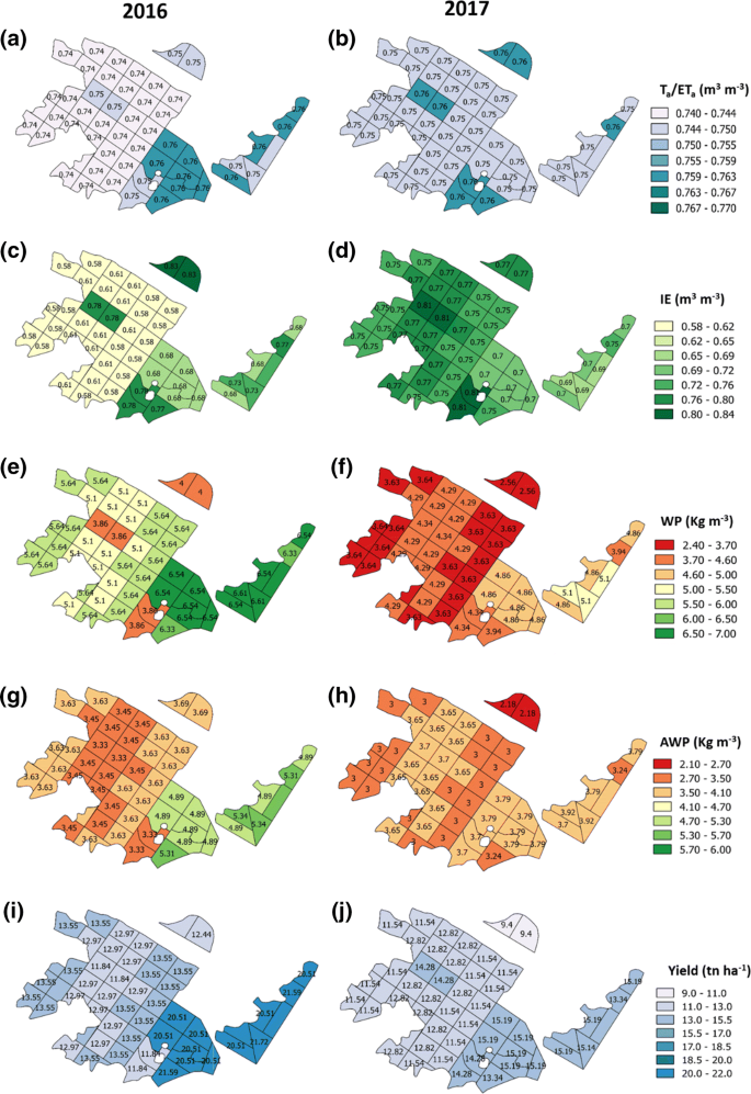
This study demonstrates the technical and economic feasibility of developing a precision irrigation management strategy for a 100-ha organic vineyard using the technological procedure of a decision-oriented vine water consumption model and remote sensing information. Despite the heterogeneity in vine water consumption between the different irrigation sectors of the vineyard, scheduling irrigation in a differential manner according to the prescriptions generated by the vine water consumption model resulted in vines with similar vine water status in all the irrigation sectors and throughout the growing season. In both years of the study, the difference between the maximum and the minimum amount of water applied in the different irrigation sectors varied by as much as 25.6%. The water savings that were achieved increased both water and energy use efficiency. When comparing a PI with a NPI strategy in terms of the amount of water needed in the vineyard, differences ranged between 14% and 38% depending on the year and water demand of the irrigation sector. Energy and water cost savings as high as 35% and 53%, respectively, were obtained with the precision irrigation strategy. It is estimated that the net economic benefit to the farmer (related to water and energy) of conducting a precision irrigation management strategy, after including all overhead expenses, amounted to 20.0 € ha −1 in 2016 and 48.7 € ha −1 in 2017. After two consecutive years of differential irrigation management, the coefficient of variability (Cv) of NDVI between irrigation sectors showed a slight declining trend, with values falling from 32.0% in 2015 to 28.4% in 2017, indicating greater homogeneity within the vineyard. It therefore seems reasonable to conclude that—taking into account the demonstrated net energy and water savings and consequent economic benefit, the associated improvement in berry composition attributes due to the adoption of RDI, as well as the trend of increased homogeneity—the adoption of PI is both necessary and profitable for most wineries. The transpiration ratio, i.e., WP and AWP of the vineyard ranged from 0.74 to 0.76 m 3 m −3 , 0.58–0.83 m 3 m −3 , 2.56–6.61 kg m −3 and from 2.18 to 5.34 kg m −3 respectively. The seasonal soil evaporation (E) accounted for 22–24% of the total amount of evapotranspiration (ETa). Yield was positively correlated to the fraction of reference evapotranspiration (ETrFnorm), but not with the NDVI. Finally, although more research is needed in this respect, it seems that the use of estimations of the biophysical parameters of the vegetation (i.e. FAPAR) using the S2 toolbox of the SNAP software could be a feasible alternative to obtaining time-series of canopy vegetative growth at spatial level, and as a consequence it will help the reduce costs related to measurements in the vines.
This research was supported by the Operational Group ‘VINECO: Profitability of applying new technologies to enhance irrigation efficiency in a 100-ha organic and conventional vineyard’ (16.01.01) funded by the Catalan Department of Agriculture (DARP) and the European Alliance for Innovation (EAI).